Country-level vulnerability assessment#
In this notebook, we will perform a vulnerability analysis for all available CI data within a country. The assessment is based on combining hazard data (e.g., flood depths) with OpenStreetMap feature data.
We will follow the steps outlined below to conduct the assessment:
Loading the necessary packages:
We will import the Python libraries required for data handling, analysis, and visualization.Loading the data:
The infrastructure data (e.g., roads) and hazard data (e.g., flood depths) will be loaded into the notebook.Preparing the data:
The infrastructure and hazard data will be processed and data gaps can be filled, if required.Performing the damage assessment:
We will overlay the hazard data with the feature information.Visualizing the results:
Finally, we will visualize the estimated exposure using graphs and maps.
1. Loading the Necessary Packages#
To perform the assessment, we are going to make use of several python packages.
In case you run this in Google Colab, you will need to install the packages below (remove the hashtag in front of them). The installation is split into two steps:
Step 1: Install damagescanner first. Because this upgrades NumPy to a newer version than what Colab has pre-installed, Google Colab will prompt you to restart the runtime after installation — accept the restart. This is necessary to ensure the newly installed NumPy version is actually loaded into memory.
Step 2: After the restart, run the second cell to install contextily. This package is installed separately to avoid the installation to fail due to the requested runtime restart.
#!pip install damagescanner
#!pip install contextily
In this step, we will import all the required Python libraries for data manipulation, spatial analysis, and visualization.
import warnings
import xarray as xr
import numpy as np
import pandas as pd
import geopandas as gpd
import seaborn as sns
import shapely
from tqdm import tqdm

import matplotlib.pyplot as plt
import contextily as cx

import damagescanner.download as download
from damagescanner.core import DamageScanner
from damagescanner.osm import read_osm_data
from damagescanner.config import DICT_CIS_VULNERABILITY_FLOOD
from statistics import mode

warnings.simplefilter(action='ignore', category=FutureWarning)
warnings.simplefilter(action='ignore', category=RuntimeWarning) # exactextract gives a warning that is invalid
Specify the country of interest#
Before we continue, we should specify the country for which we want to assess the damage. We use the ISO3 code for the country to download the OpenStreetMap data.
country_full_name = 'Burkina Faso'
country_iso3 = 'BFA'
2. Loading the Data#
In this step, we will prepare and load two key datasets:
Infrastructure data:
This dataset contains information on the location and type of infrastructure (e.g., roads). Each asset may have attributes such as type, length, and replacement cost.Hazard data:
This dataset includes information on the hazard affecting the infrastructure (e.g., flood depth at various locations).
Infrastructure Data#
We will perform this example analysis for Jamaica. To start the analysis, we first download the OpenStreetMap data from GeoFabrik.
infrastructure_path = download.get_country_geofabrik(country_iso3)
We will not load the data directly, we will let the code itself read the information. It is important, however, to specificy which infrastructure systems you want to include. We do so in the list below:
asset_types = [
        "roads",
        "rail",
        "air",
        "telecom",
        "water_supply",
        "waste_solid",
        "waste_water",
        "education",
        "healthcare",
        "power",
    ]
Vulnerability data#
We will collect all the vulnerability curves for each of the asset types. Important to note is that national or local-scale analysis requires a thorough check which curves can and should be used!
vulnerability_path = "https://zenodo.org/records/10203846/files/Table_D2_Multi-Hazard_Fragility_and_Vulnerability_Curves_V1.0.0.xlsx?download=1"

vul_df = pd.read_excel(vulnerability_path,sheet_name='F_Vuln_Depth')
damage_curves_all_ci = {}
for ci_type in DICT_CIS_VULNERABILITY_FLOOD:

    ci_system = DICT_CIS_VULNERABILITY_FLOOD[ci_type]

    selected_curves = []
    for subtype in ci_system:
        selected_curves.append(ci_system[subtype][0])

    damage_curves = vul_df[['ID number']+selected_curves]
    damage_curves = damage_curves.iloc[4:125,:]
    damage_curves.set_index('ID number',inplace=True)
    damage_curves.index = damage_curves.index.rename('Depth')
    damage_curves = damage_curves.astype(np.float32)
    damage_curves.columns = list(ci_system.keys())
    damage_curves = damage_curves.ffill()

    # Make sure we set the index of the damage curves (the inundation depth) in the same metric as the hazard data (e.g. meters or centimeters).
    damage_curves.index = damage_curves.index*100

    damage_curves_all_ci[ci_type] = damage_curves
Maximum damages#
One of the most difficult parts of the assessment is to define the maximum reconstruction cost of particular assets. As such, we sometimes may want to run the analysis without already multiplying the results with those costs. To do so, we simply set all the maximum damage values to 1:
maxdam_all_ci = {}
for ci_type in DICT_CIS_VULNERABILITY_FLOOD:
    ci_system = DICT_CIS_VULNERABILITY_FLOOD[ci_type]
    maxdam_dict = dict(zip(list(ci_system.keys()),len(ci_system.keys())*[1]))
    maxdam = pd.DataFrame.from_dict(maxdam_dict,orient='index').reset_index()
    maxdam.columns = ['object_type','damage']
    maxdam_all_ci[ci_type] =  maxdam
Hazard Data#
For this example, we make use of the flood data provided by CDRI.
We use a 1/100 flood map to showcase the approach.
hazard_map = xr.open_dataset("https://hazards-data.unepgrid.ch/global_pc_h100glob.tif", engine="rasterio")
Ancilliary data for processing#
world = gpd.read_file("https://github.com/nvkelso/natural-earth-vector/raw/master/10m_cultural/ne_10m_admin_0_countries.shp")
world_plot = world.to_crs(3857)
3. Preparing the Data#
Clip the hazard data to the country of interest.
country_bounds = world.loc[world.ADM0_ISO == country_iso3].bounds
country_geom = world.loc[world.ADM0_ISO == country_iso3].geometry
country_box = shapely.box(country_bounds.minx.values,country_bounds.miny.values,country_bounds.maxx.values,country_bounds.maxy.values)[0]
hazard_country = hazard_map.rio.clip_box(minx=country_bounds.minx.values[0],
                     miny=country_bounds.miny.values[0],
                     maxx=country_bounds.maxx.values[0],
                     maxy=country_bounds.maxy.values[0]
                    )
4. Performing the Vulnerability Assessment#
We will use the DamageScanner approach. This is a fully optimised exposure, vulnerability damage and risk calculation method, that can capture a wide range of inputs to perform such an assessment.
save_asset_results = {}
for asset_type in asset_types:
    try:
        save_asset_results[asset_type] = DamageScanner(hazard_country,
                                                       infrastructure_path,
                                                       curves=damage_curves_all_ci[asset_type],
                                                       maxdam=maxdam_all_ci[asset_type]).calculate(
            asset_type=asset_type
        )
    except:
        print(f"It seems that {asset_type} is most likely not mapped or has no exposure")
Overlay raster with vector: 100%|████████████████████████████████████████████████████| 192/192 [00:53<00:00,  3.58it/s]
convert coverage to meters: 100%|███████████████████████████████████████████| 190621/190621 [00:18<00:00, 10246.58it/s]
Calculating damage: 100%|████████████████████████████████████████████████████| 190621/190621 [00:28<00:00, 6756.81it/s]
Overlay raster with vector: 100%|████████████████████████████████████████████████████| 192/192 [00:02<00:00, 74.32it/s]
convert coverage to meters: 100%|██████████████████████████████████████████████████| 505/505 [00:00<00:00, 7326.87it/s]
Calculating damage: 100%|██████████████████████████████████████████████████████████| 505/505 [00:00<00:00, 7497.33it/s]
Overlay raster with vector: 100%|████████████████████████████████████████████████████| 192/192 [00:02<00:00, 74.04it/s]
convert coverage to meters: 100%|████████████████████████████████████████████████████| 64/64 [00:00<00:00, 8179.27it/s]
Calculating damage: 100%|████████████████████████████████████████████████████████████| 64/64 [00:00<00:00, 4297.72it/s]
Overlay raster with vector: 100%|████████████████████████████████████████████████████| 192/192 [00:04<00:00, 47.99it/s]
convert coverage to meters: 100%|█████████████████████████████████████████████████| 555/555 [00:00<00:00, 26016.64it/s]
Calculating damage: 100%|██████████████████████████████████████████████████████████| 555/555 [00:00<00:00, 5862.76it/s]
Overlay raster with vector: 100%|████████████████████████████████████████████████████| 192/192 [00:02<00:00, 70.11it/s]
convert coverage to meters: 100%|█████████████████████████████████████████████| 10689/10689 [00:00<00:00, 31015.36it/s]
Calculating damage: 100%|██████████████████████████████████████████████████████| 10689/10689 [00:01<00:00, 7190.15it/s]
Overlay raster with vector: 100%|███████████████████████████████████████████████████| 192/192 [00:01<00:00, 109.99it/s]
convert coverage to meters: 100%|██████████████████████████████████████████████████████| 2/2 [00:00<00:00, 1759.36it/s]
Calculating damage: 100%|██████████████████████████████████████████████████████████████| 2/2 [00:00<00:00, 1290.75it/s]
Overlay raster with vector: 100%|████████████████████████████████████████████████████| 192/192 [00:06<00:00, 28.55it/s]
convert coverage to meters: 100%|███████████████████████████████████████████████| 5456/5456 [00:00<00:00, 24425.44it/s]
Calculating damage: 100%|████████████████████████████████████████████████████████| 5456/5456 [00:01<00:00, 4520.47it/s]
Overlay raster with vector: 100%|████████████████████████████████████████████████████| 192/192 [00:03<00:00, 55.15it/s]
convert coverage to meters: 100%|███████████████████████████████████████████████| 1159/1159 [00:00<00:00, 30516.95it/s]
Calculating damage: 100%|████████████████████████████████████████████████████████| 1159/1159 [00:00<00:00, 7170.48it/s]
Overlay raster with vector: 100%|████████████████████████████████████████████████████| 192/192 [00:03<00:00, 60.38it/s]
convert coverage to meters: 100%|█████████████████████████████████████████████| 15074/15074 [00:00<00:00, 25512.39it/s]
Calculating damage: 100%|██████████████████████████████████████████████████████| 15074/15074 [00:01<00:00, 7612.96it/s]
5. Visualising the results#
collect_damages = {}
for asset_type in asset_types:
    damage_results = save_asset_results[asset_type]
    if len(damage_results) == 0:
        continue
    else:
        collect_damages[asset_type] = damage_results.damage.sum()
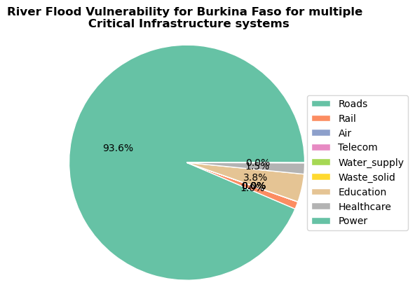
colors = ['#66c2a5','#fc8d62','#8da0cb','#e78ac3','#a6d854','#ffd92f','#e5c494','#b3b3b3']
labels = [x.capitalize() for x in list(collect_damages.keys())]
sizes = collect_damages.values()
pie = plt.pie(sizes,autopct='%1.1f%%', labeldistance=1.15, wedgeprops = { 'linewidth' : 1, 'edgecolor' : 'white' }, colors=colors);
plt.axis('equal')
plt.legend(loc = 'right', labels=labels,bbox_to_anchor=(1.15, 0.5),)
plt.title(f'River Flood Vulnerability for {country_full_name} for multiple \n Critical Infrastructure systems',fontweight='bold')
Text(0.5, 1.0, 'River Flood Vulnerability for Burkina Faso for multiple \n Critical Infrastructure systems')