Tropical Cyclone Risk Assessment#
In this notebook, we will perform a tropical cyclone damage and risk assessment for education infrastructure. The assessment is based on combining hazard data (e.g., flood depths) with vulnerability curves to estimate the potential damage to infrastructure.
We will follow the steps outlined below to conduct the assessment:
Loading the necessary packages:
We will import the Python libraries required for data handling, analysis, and visualization.Loading the data:
The infrastructure data (e.g., secondary schools) and hazard data (e.g., flood depths) will be loaded into the notebook.Preparing the data:
The infrastructure and hazard data will be processed and data gaps can be filled, if required.Performing the damage assessment:
We will apply vulnerability curves to estimate the potential damage based on the intensity of the hazard.Visualizing the results:
Finally, we will visualize the estimated damage using graphs and maps to illustrate the impact on education infrastructure.
1. Loading the Necessary Packages#
To perform the assessment, we are going to make use of several python packages.
In case you run this in Google Colab, you will need to install the packages below (remove the hashtag in front of them). The installation is split into two steps:
Step 1: Install damagescanner first. Because this upgrades NumPy to a newer version than what Colab has pre-installed, Google Colab will prompt you to restart the runtime after installation — accept the restart. This is necessary to ensure the newly installed NumPy version is actually loaded into memory.
Step 2: After the restart, run the second cell to install contextily. This package is installed separately to avoid the installation to fail due to the requested runtime restart.
#!pip install damagescanner
#!pip install contextily
In this step, we will import all the required Python libraries for data manipulation, spatial analysis, and visualization.
import warnings
import xarray as xr
import numpy as np
import pandas as pd
import geopandas as gpd
import seaborn as sns
import shapely

import matplotlib.pyplot as plt
import contextily as cx

import damagescanner.download as download
from damagescanner.core import DamageScanner
from damagescanner.osm import read_osm_data
from damagescanner.config import DICT_CIS_VULNERABILITY_FLOOD

warnings.simplefilter(action='ignore', category=FutureWarning)
warnings.simplefilter(action='ignore', category=RuntimeWarning) # exactextract gives a warning that is invalid
Specify the country of interest#
Before we continue, we should specify the country for which we want to assess the damage. We use the ISO3 code for the country to download the OpenStreetMap data.
country_full_name = 'Vietnam'
country_iso3 = 'VNM'
2. Loading the Data#
In this step, we will load four key datasets:
Infrastructure data:
This dataset contains information on the location and type of transportation infrastructure (e.g., roads). Each asset may have attributes such as type, length, and replacement cost.Hazard data:
This dataset includes information on the hazard affecting the infrastructure (e.g., flood depth at various locations).Vulnerability curves:
Vulnerability curves define how the infrastructure’s damage increases with the intensity of the hazard. For example, flood depth-damage curves specify how much damage occurs for different flood depths.Maximum damage values:
This dataset contains the maximum possible damage (in monetary terms) that can be incurred by individual infrastructure assets. This is crucial for calculating total damage based on the vulnerability curves.
Infrastructure Data#
We will perform this example analysis for Jamaica. To start the analysis, we first download the OpenStreetMap data from GeoFabrik.
infrastructure_path = download.get_country_geofabrik(country_iso3)
Now we load the data and read only the education data.
%%time
features = read_osm_data(infrastructure_path,asset_type='education')
CPU times: total: 1min 18s
Wall time: 2min 30s
sub_types = features.object_type.unique()
sub_types
<ArrowStringArray>
['school', 'kindergarten', 'library', 'college', 'university']
Length: 5, dtype: str
And we can explore our data interactively
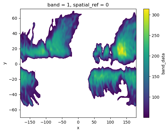
Hazard Data#
For this example, we make use of the flood data provided by CDRI.
We use a 1/250 Tropical Cyclone wind speed map to showcase the approach.
hazard_map = xr.open_dataset("https://hazards-data.unepgrid.ch/Wind_T250.tif", engine="rasterio")
hazard_map.band_data.plot()
<matplotlib.collections.QuadMesh at 0x26e338c9940>
Maximum damages#
One of the most difficult parts of the assessment is to define the maximum reconstruction cost of particular assets. Here we provide a baseline set of values, but these should be updated through national consultations.
Locations of education facilities are (somewhat randomly) geotagged as either points or polygons. This matters quite a lot for the maximum damages. For polygons, we would use damage per square meter, whereas for points, we would estimate the damage to the entire asset at once. Here we take the approach of converting the points to polygons, and there define our maximum damages in dollar per square meter.
maxdam_dict = {'community_centre' : 1000,
               'school' : 1000,
               'kindergarten' : 1000,
               'university' : 1000,
               'college' : 1000,
               'library' : 1000
              }
To be used in our damage assessment, we convert this to a Pandas DataFrame
maxdam = pd.DataFrame.from_dict(maxdam_dict,orient='index').reset_index()
maxdam.columns = ['object_type','damage']
And check if any of the objects are missing from the dataframe.
missing = set(sub_types) - set(maxdam.object_type)

if len(missing) > 0:
    print(f"Missing object types in maxdam: \033[1m{', '.join(missing)}\033[0m. Please add them before you continue.")
Vulnerability data#
Similarly to the maximum damages, specifying the vulnerability curves is complex. We generally have limited information about the quality of the assets, its level of deteriation and other asset-level characteristics.
vulnerability_path = "https://zenodo.org/records/13889558/files/Table_D2_Hazard_Fragility_and_Vulnerability_Curves_V1.1.0.xlsx?download=1"
vul_df = pd.read_excel(vulnerability_path,sheet_name='W_Vuln_V10m')
And let’s have a look at all the available options
with pd.option_context('display.max_rows', None, 'display.max_colwidth', None):
  display(vul_df.iloc[:2,:].T)
| 0 | 1 | |
|---|---|---|
| ID number | Infrastructure description | Additional characteristics |
| W1.1 | Windturbine | 1-MW capacity, 40-m hub height |
| W1.1a | Windturbine | 1-MW capacity, 40-m hub height |
| W1.1b | Windturbine | 1-MW capacity, 40-m hub height |
| W1.2 | Windturbine | 2.5-MW capacity, 80-m hub height |
| W1.2a | Windturbine | 2.5-MW capacity, 80-m hub height |
| W1.2b | Windturbine | 2.5-MW capacity, 80-m hub height |
| W1.3 | Windturbine | 3.3-MW capacity, 100-m hub height |
| W1.3a | Windturbine | 3.3-MW capacity, 100-m hub height |
| W1.3b | Windturbine | 3.3-MW capacity, 100-m hub height |
| W3.5 | Power tower | Design speed 110 km/h, urban terrain |
| W3.6 | Power tower | Design speed 120 km/h, urban terrain |
| W3.7 | Power tower | Design speed 130 km/h, urban terrain |
| W3.8 | Power tower | Design speed 140 km/h, urban terrain |
| W3.9 | Power tower | Design speed 150 km/h, urban terrain |
| W3.10 | Power tower | Design speed 160 km/h, urban terrain |
| W3.11 | Power tower | Design speed 170 km/h, urban terrain |
| W3.12 | Power tower | Design speed 180 km/h, urban terrain |
| W3.13 | Power tower | Design speed 190 km/h, urban terrain |
| W3.14 | Power tower | Design speed 200 km/h, urban terrain |
| W7.2 | Roads | NaN |
| W14.1 | Water treatment plant | NaN |
| W16.1 | Transmission and distribution pipelines | Buried pipelines |
| W18.1 | Wastewater treatment plant | NaN |
| W19.1 | Sewers & interceptors | Buried pipelines |
| W21.1 | School | Building design: Marcos |
| W21.2 | School | Building design: BLSB1 |
| W21.3 | School | Building design: RPUS |
| W21.4 | School | Building design: DECS std. |
| W21.5 | School | Building design: DepEd STD |
| W21.10 | School | Wooden roof structure |
| W21.10a | School | Wooden roof structure |
| W21.10b | School | Wooden roof structure |
As we do not exactly know which curves we may want to use, we can also run the analysis with all curves. To do so, we select all education-related curves from Nirandjan et al. (2024)’s database.
selected_curves = ['W21.2','W21.3','W21.4','W21.5','W21.10']
The next step is to extract the curves from the database, and prepare them for proper usage into our analysis.
We start by selecting the curve IDs from the larger pandas DataFrame vul_df:
damage_curves = vul_df[['ID number']+selected_curves]
damage_curves = damage_curves.iloc[4:125,:]
Then for convenience, we rename the index name to the hazard intensity we are considering.
damage_curves.set_index('ID number',inplace=True)
damage_curves.index = damage_curves.index.rename('WindSpeed')
And make sure that our damage values are in floating numbers.
damage_curves = damage_curves.astype(np.float32)
And ensure that the columns of the curves link back to the different asset types we are considering:
damage_curves.columns = sub_types
There could be some NaN values at the tail of some of the curves. To make sure the code works, we fill up the NaN values with the last value of each of the curves.
damage_curves = damage_curves.ffill()
And check if any of the objects are missing from the dataframe.
But in some cases, we do not exactly know which curves we may want to use. As such, we can also run the analysis with all curves. To do so, we select all education-related curves from Nirandjan et al. (2024)’s database.
unique_curves = ['W21.1','W21.2','W21.3','W21.4','W21.5','W21.10']
And create a dictionary that contains a pandas DataFrame for all object types, for each vulnerability curve.
multi_curves = {}
for unique_curve in unique_curves:

    curve_creation = damage_curves.copy()

    get_curve_values = vul_df[unique_curve].iloc[4:125].values.astype(np.float32)

    for curve in curve_creation:
        curve_creation.loc[:,curve] = get_curve_values

    multi_curves[unique_curve] = curve_creation.astype(np.float32).ffill()
Ancilliary data for processing#
world = gpd.read_file("https://github.com/nvkelso/natural-earth-vector/raw/master/10m_cultural/ne_10m_admin_0_countries.shp")
world_plot = world.to_crs(3857)
admin1 = gpd.read_file("https://github.com/nvkelso/natural-earth-vector/raw/master/10m_cultural/ne_10m_admin_1_states_provinces.shp")
3. Preparing the Data#
Clip the hazard data to the country of interest.
country_bounds = world.loc[world.ADM0_ISO == country_iso3].bounds
country_geom = world.loc[world.ADM0_ISO == country_iso3].geometry
hazard_country = hazard_map.rio.clip_box(minx=country_bounds.minx.values[0],
                     miny=country_bounds.miny.values[0],
                     maxx=country_bounds.maxx.values[0],
                     maxy=country_bounds.maxy.values[0]
                    )
Convert point data to polygons.#
For some data, there are both points and polygons available. It makes life easier to estimate the damage using polygons. Therefore, we convert those points to Polygons below.
Let’s first get an overview of the different geometry types for all the assets we are considering in this analysis:
features['geom_type'] = features.geom_type
features.groupby(['object_type','geom_type']).count()['geometry']
object_type   geom_type
college       MultiPolygon     498
              Point             64
kindergarten  MultiPolygon    1216
              Point            284
library       MultiPolygon      57
              Point             29
school        MultiPolygon    6294
              Point           1436
university    MultiPolygon     436
              Point             27
Name: geometry, dtype: int64
The results above indicate that several asset types that are expected to be Polygons are stored as Points as well. It would be preferably to convert them all to polygons. For the Points, we will have to estimate a the average size, so we can use that to create a buffer around the assets.
To do so, let’s grab the polygon data and estimate their size. We grab the median so we are not too much influenced by extreme outliers. If preferred, please change .median() to .mean() (or any other metric).
polygon_features = features.loc[features.geometry.geom_type.isin(['Polygon','MultiPolygon'])].to_crs(3857)
polygon_features['square_m2'] = polygon_features.area

square_m2_object_type = polygon_features[['object_type','square_m2']].groupby('object_type').median()
square_m2_object_type
| square_m2 | |
|---|---|
| object_type | |
| college | 23175.745744 |
| kindergarten | 3633.040315 |
| library | 1165.687415 |
| school | 8156.883968 |
| university | 38093.105077 |
Now we create a list in which we define the assets we want to “polygonize”:
points_to_polygonize = ['college','kindergarten','library','school','university']
And take them from our data again:
all_assets_to_polygonize = features.loc[(features.object_type.isin(points_to_polygonize)) & (features.geometry.geom_type == 'Point')]
When performing a buffer, it is always best to do this in meters. As such, we will briefly convert the point data into a crs system in meters.
all_assets_to_polygonize = all_assets_to_polygonize.to_crs(3857)
def polygonize_point_per_asset(asset):

    # we first need to set a buffer length. This is half of width/length of an asset.
    buffer_length = np.sqrt(square_m2_object_type.loc[asset.object_type].values[0])/2

    # then we can buffer the asset
    return asset.geometry.buffer(buffer_length,cap_style='square')

collect_new_point_geometries = all_assets_to_polygonize.apply(lambda asset:  polygonize_point_per_asset(asset),axis=1).set_crs(3857).to_crs(4326).values
features.loc[(features.object_type.isin(points_to_polygonize)) & (features.geometry.geom_type == 'Point'),'geometry'] = collect_new_point_geometries
And check if any “undesired” Points are still left:
features.loc[(features.object_type.isin(points_to_polygonize)) & (features.geometry.geom_type == 'Point')]
| osm_id | geometry | object_type | building | name | geom_type |
|---|
And remove the ‘geom_type’ column again, as we do not need it again.
5. Performing the Damage Assessment#
We will use the DamageScanner approach. This is a fully optimised damage calculation method, that can capture a wide range of inputs to perform a damage assessment. We will first perform this using only a single damage curve.
%%time
damage_results = DamageScanner(hazard_country, features, damage_curves, maxdam).calculate(disable_progress=False)
Overlay raster with vector: 100%|████████████████████████████████████████████████████| 480/480 [00:11<00:00, 42.44it/s]
convert coverage to meters: 100%|█████████████████████████████████████████████| 10341/10341 [00:00<00:00, 20205.95it/s]
Calculating damage: 100%|██████████████████████████████████████████████████████| 10341/10341 [00:01<00:00, 5875.94it/s]
CPU times: total: 5.95 s
Wall time: 15 s
And run this also with the range of vulnerability curves.
%%time
all_results = DamageScanner(hazard_country, features, damage_curves, maxdam).calculate(multi_curves=multi_curves)
Overlay raster with vector: 100%|████████████████████████████████████████████████████| 480/480 [00:09<00:00, 49.73it/s]
convert coverage to meters: 100%|█████████████████████████████████████████████| 10341/10341 [00:00<00:00, 16786.79it/s]
Calculating damage: 100%|██████████████████████████████████████████████████████| 10341/10341 [00:01<00:00, 5438.88it/s]
Calculating damage: 100%|██████████████████████████████████████████████████████| 10341/10341 [00:01<00:00, 7406.82it/s]
Calculating damage: 100%|██████████████████████████████████████████████████████| 10341/10341 [00:01<00:00, 7119.43it/s]
Calculating damage: 100%|██████████████████████████████████████████████████████| 10341/10341 [00:01<00:00, 7333.26it/s]
Calculating damage: 100%|██████████████████████████████████████████████████████| 10341/10341 [00:01<00:00, 7600.44it/s]
Calculating damage: 100%|██████████████████████████████████████████████████████| 10341/10341 [00:01<00:00, 7732.80it/s]
CPU times: total: 8.31 s
Wall time: 20.8 s
5. Save the Results#
For further analysis, we can save the results in their full detail, or save summary estimates per subnational unit
hazard = 'tropical_cyclones'
return_period = '1_250'
damage_results.to_file(f'Education_Damage_{country_full_name}_{hazard}_{return_period}.gpkg')
admin1_country = admin1.loc[admin1.sov_a3 == country_iso3]
damage_results = damage_results.sjoin(admin1_country[['adm1_code','name','geometry']])
6. Visualizing the Results#
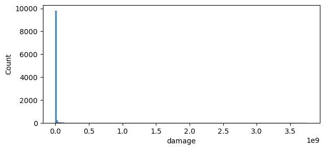
The results of the damage assessment can be visualized using charts and maps. This will provide a clear representation of which infrastructure is most affected by the hazard and the expected damage levels.
And create a distribution of the damages.
fig, ax = plt.subplots(1,1,figsize=(7, 3))

sns.histplot(data=damage_results,x='damage',ax=ax)
<Axes: xlabel='damage', ylabel='Count'>
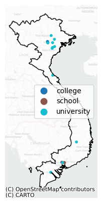
Plot location of most damaged healthcare facilities
fig, ax = plt.subplots(1,1,figsize=(10, 5))

subset = damage_results.to_crs(3857).sort_values('damage',ascending=False).head(20)
subset.geometry = subset.centroid
subset.plot(ax=ax,column='object_type',markersize=10,legend=True)
world_plot.loc[world.SOV_A3 == country_iso3].plot(ax=ax,facecolor="none",edgecolor='black')
cx.add_basemap(ax, source=cx.providers.CartoDB.Positron,alpha=0.5)
ax.set_axis_off()
7. Performing the Risk Assessment#
To do so, we need to select the return periods we want to include, and create a dictioniary as input. We will create this below.
return_periods = [25,50,100,250]

hazard_dict = {}
collect_max_pres = []
for return_period in return_periods:
    hazard_map = xr.open_dataset(f"https://hazards-data.unepgrid.ch/Wind_T{return_period}.tif", engine="rasterio")

    hazard_dict[return_period] = hazard_map.rio.clip_box(minx=country_bounds.minx.values[0],
                     miny=country_bounds.miny.values[0],
                     maxx=country_bounds.maxx.values[0],
                     maxy=country_bounds.maxy.values[0]
                    )
    collect_max_pres.append(hazard_map.band_data.max().values)
And below we will run a multi-curve risk assessment.
risk_results = DamageScanner(hazard_country, features, damage_curves, maxdam).risk(hazard_dict,multi_curves=multi_curves)
Risk Calculation: 100%|██████████████████████████████████████████████████████████████████| 4/4 [01:02<00:00, 15.68s/it]
7. Performing the Risk Assessment under Climate Change#
To do so, we need to select the return periods we want to include, and create a dictioniary as input. We will create this below.
return_periods = [25,50,100,250]

hazard_dict_future = {}
collect_max = []
for return_period in return_periods:
    hazard_map = xr.open_dataset(f"https://hazards-data.unepgrid.ch/Wind_CC_T{return_period}.tif", engine="rasterio")

    hazard_dict_future[return_period] = hazard_map.rio.clip_box(minx=country_bounds.minx.values[0],
                     miny=country_bounds.miny.values[0],
                     maxx=country_bounds.maxx.values[0],
                     maxy=country_bounds.maxy.values[0]
                    )
    collect_max.append(hazard_map.band_data.max().values)
risk_results_future = DamageScanner(hazard_country, features, damage_curves, maxdam).risk(hazard_dict_future,multi_curves=multi_curves)
Risk Calculation: 100%|██████████████████████████████████████████████████████████████████| 4/4 [01:02<00:00, 15.53s/it]
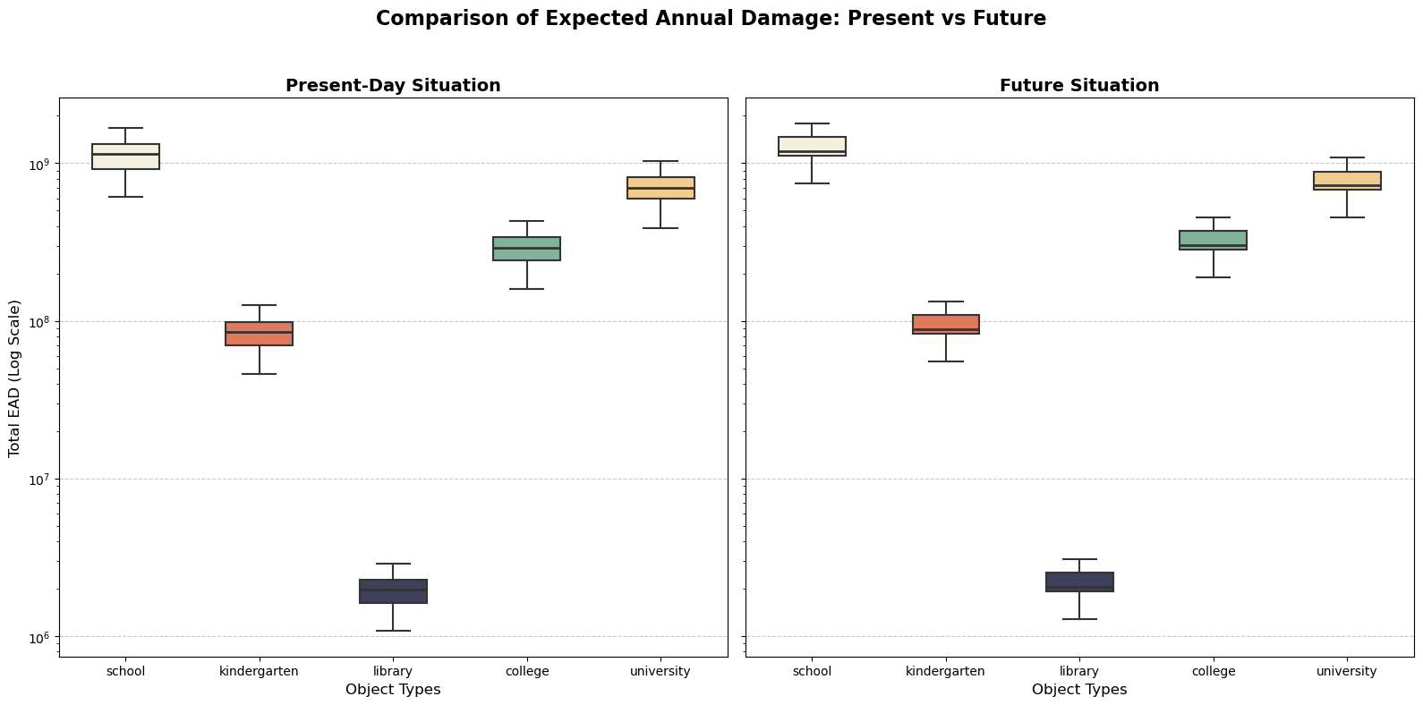
8. Visualize the risk results#
# Create a figure with 2 subplots (2 rows, 1 column)
fig, axes = plt.subplots(1, 2, figsize=(16, 8), sharey=True)

# Define line color and colors for boxes
colors = ['#f4f1de', '#e07a5f', '#3d405b', '#81b29a', '#f2cc8f']
line_color = '#333333'

# --- Left plot: Present day ---
grouped_present = risk_results[['object_type'] + unique_curves].groupby('object_type').sum()
boxplot_present = grouped_present.T.boxplot(column=list(sub_types), grid=False, patch_artist=True, ax=axes[0], return_type='dict')

# Customize present day plot
for box, color in zip(boxplot_present['boxes'], colors):
    box.set_facecolor(color)
    box.set_edgecolor(line_color)
    box.set_linewidth(1.5)

for whisker in boxplot_present['whiskers']:
    whisker.set_color(line_color)
    whisker.set_linewidth(1.5)

for cap in boxplot_present['caps']:
    cap.set_color(line_color)
    cap.set_linewidth(1.5)

for median in boxplot_present['medians']:
    median.set_color(line_color)
    median.set_linewidth(2)

for flier in boxplot_present['fliers']:
    flier.set_markerfacecolor(line_color)
    flier.set_markeredgecolor(line_color)

axes[0].set_title('Present-Day Situation', fontsize=14, fontweight='bold')
axes[0].set_ylabel('Total EAD (Log Scale)', fontsize=12)
axes[0].set_xlabel('Object Types', fontsize=12)
axes[0].set_yscale('log')
axes[0].grid(axis='y', linestyle='--', alpha=0.7)
axes[0].tick_params(axis='x', rotation=0, labelsize=10)
axes[0].tick_params(axis='y', labelsize=10)

# --- Right plot: Future situation ---
grouped_future = risk_results_future[['object_type'] + unique_curves].groupby('object_type').sum()
boxplot_future = grouped_future.T.boxplot(column=list(sub_types), grid=False, patch_artist=True, ax=axes[1], return_type='dict')

# Customize future plot
for box, color in zip(boxplot_future['boxes'], colors):
    box.set_facecolor(color)
    box.set_edgecolor(line_color)
    box.set_linewidth(1.5)

for whisker in boxplot_future['whiskers']:
    whisker.set_color(line_color)
    whisker.set_linewidth(1.5)

for cap in boxplot_future['caps']:
    cap.set_color(line_color)
    cap.set_linewidth(1.5)

for median in boxplot_future['medians']:
    median.set_color(line_color)
    median.set_linewidth(2)

for flier in boxplot_future['fliers']:
    flier.set_markerfacecolor(line_color)
    flier.set_markeredgecolor(line_color)

axes[1].set_title('Future Situation', fontsize=14, fontweight='bold')
axes[1].set_xlabel('Object Types', fontsize=12)
axes[1].grid(axis='y', linestyle='--', alpha=0.7)
axes[1].tick_params(axis='x', rotation=0, labelsize=10)

# Add overall title
fig.suptitle('Comparison of Expected Annual Damage: Present vs Future', fontsize=16, fontweight='bold')

# Adjust layout to prevent overlap
plt.tight_layout(rect=[0, 0, 1, 0.95])

# Show the plot
plt.show()