Earthquake Damage Assessment#
In this notebook, we will perform an earthquake damage and risk assessment for transportation infrastructure, specifically focusing on roads. The assessment is based on combining hazard data (e.g., PGA levels) with vulnerability curves to estimate the potential damage to infrastructure.
We will follow the steps outlined below to conduct the assessment:
Loading the necessary packages:
We will import the Python libraries required for data handling, analysis, and visualization.Loading the data:
The infrastructure data (e.g., roads) and hazard data (e.g., PGA levels) will be loaded into the notebook.Preparing the data:
The infrastructure and hazard data will be processed and data gaps can be filled, if required.Performing the damage assessment:
We will apply vulnerability curves to estimate the potential damage based on the intensity of the hazard.Visualizing the results:
Finally, we will visualize the estimated damage using graphs and maps to illustrate the impact on transportation infrastructure.
1. Loading the Necessary Packages#
To perform the assessment, we are going to make use of several python packages.
In case you run this in Google Colab, you will need to install the packages below (remove the hashtag in front of them). The installation is split into two steps:
Step 1: Install damagescanner first. Because this upgrades NumPy to a newer version than what Colab has pre-installed, Google Colab will prompt you to restart the runtime after installation — accept the restart. This is necessary to ensure the newly installed NumPy version is actually loaded into memory.
Step 2: After the restart, run the second cell to install contextily. This package is installed separately to avoid the installation to fail due to the requested runtime restart.
#!pip install damagescanner
#!pip install contextily
In this step, we will import all the required Python libraries for data manipulation, spatial analysis, and visualization.
import warnings
import xarray as xr
import numpy as np
import pandas as pd
import geopandas as gpd
import seaborn as sns
import shapely
from tqdm import tqdm

import matplotlib.pyplot as plt
import contextily as cx

import damagescanner.download as download
from damagescanner.core import DamageScanner
from damagescanner.osm import read_osm_data
from damagescanner.config import DICT_CIS_VULNERABILITY_FLOOD
from statistics import mode


warnings.simplefilter(action='ignore', category=FutureWarning)
warnings.simplefilter(action='ignore', category=RuntimeWarning) # exactextract gives a warning that is invalid
Specify the country of interest#
Before we continue, we should specify the country for which we want to assess the damage. We use the ISO3 code for the country to download the OpenStreetMap data.
country_full_name = 'Tajikistan'
country_iso3 = 'TJK'
2. Loading the Data#
In this step, we will load four key datasets:
Infrastructure data:
This dataset contains information on the location and type of transportation infrastructure (e.g., roads). Each asset may have attributes such as type, length, and replacement cost.Hazard data:
This dataset includes information on the hazard affecting the infrastructure (e.g., flood depth at various locations).Vulnerability curves:
Vulnerability curves define how the infrastructure’s damage increases with the intensity of the hazard. For example, flood depth-damage curves specify how much damage occurs for different flood depths.Maximum damage values:
This dataset contains the maximum possible damage (in monetary terms) that can be incurred by individual infrastructure assets. This is crucial for calculating total damage based on the vulnerability curves.
Infrastructure Data#
We will perform this example analysis for Tajikistan. To start the analysis, we first download the OpenStreetMap data from GeoFabrik. In case of locally available data, one can load the shapefiles through gpd.read_file(), as we show in the second cell within this section.
infrastructure_path = download.get_country_geofabrik(country_iso3)
Now we load the data and read only the road data.
%%time
features = read_osm_data(infrastructure_path,asset_type='roads')
CPU times: total: 5.52 s
Wall time: 8.94 s
sub_types = features.object_type.unique()
sub_types
<ArrowStringArray>
[       'primary',          'trunk',          'track',       'tertiary',
      'secondary', 'secondary_link',    'residential',   'primary_link',
     'trunk_link',   'unclassified',  'tertiary_link',           'road']
Length: 12, dtype: str
Hazard Data#
For this example, we make use of the flood data provided by CDRI.
We use a 1/475 earthquake hazard map to showcase the approach.
hazard_map = xr.open_dataset("https://hazards-data.unepgrid.ch/PGA_475y.tif", engine="rasterio")
Maximum damages#
One of the most difficult parts of the assessment is to define the maximum reconstruction cost of particular assets. Here we provide a baseline set of values, but these should be updated through national consultations.
maxdam_dict = {'trunk':2000,
               'motorway' : 2000,
                'primary':2000,
                'secondary':1300,
                'tertiary':700,
                'trunk_link': 1300,
                'motorway_link' : 1300,
                'primary_link' : 1300,
               'secondary_link' : 700,
               'tertiary_link' : 700,
               'track' : 300,
               'unclassified' : 300,
               'road' : 300,
               'residential' : 300
              }
To be used in our damage assessment, we convert this to a Pandas DataFrame
maxdam = pd.DataFrame.from_dict(maxdam_dict,orient='index').reset_index()
maxdam.columns = ['object_type','damage']
And check if any of the objects are missing from the dataframe.
missing = set(sub_types) - set(maxdam.object_type)

if len(missing) > 0:
    print(f"Missing object types in maxdam: \033[1m{', '.join(missing)}\033[0m. Please add them before you continue.")
Vulnerability data#
Similarly to the maximum damages, specifying the vulnerability curves is complex. We generally have limited information about the quality of the assets, its level of deteriation and other asset-level characteristics. The study by Nirandjan et al. (2024) provides us with a baseline set of fragility and vulnerability curves that one can use. In the following cell, we load that data.
vulnerability_path = "https://zenodo.org/records/13889558/files/Table_D2_Hazard_Fragility_and_Vulnerability_Curves_V1.1.0.xlsx?download=1"
vul_df = pd.read_excel(vulnerability_path,sheet_name='E_Vuln_PGA ')
And let’s have a look at all the available options
with pd.option_context('display.max_rows', None, 'display.max_colwidth', None):
  display(vul_df.iloc[:2,:].T)
| 0 | 1 | |
|---|---|---|
| ID number | Infrastructure type | Infrastructure type details |
| E1.1 | Power plant | Small generation facilities with anchored components |
| E1.1a | Power plant | Small generation facilities with anchored components |
| E1.1b | Power plant | Small generation facilities with anchored components |
| E1.2 | Power plant | Small generation facilities with unanchored components |
| E1.2a | Power plant | Small generation facilities with unanchored components |
| E1.2b | Power plant | Small generation facilities with unanchored components |
| E1.3 | Power plant | Medium/large power with anchored components |
| E1.3a | Power plant | Medium/large power with anchored components |
| E1.3b | Power plant | Medium/large power with anchored components |
| E1.4 | Power plant | Medium/large power with unanchored components |
| E1.4a | Power plant | Medium/large power with unanchored components |
| E1.4b | Power plant | Medium/large power with unanchored components |
| E1.15 | Hydropower plants | NaN |
| E2.1 | substation | Low Voltage Substation anchored |
| E2.1a | substation | Low Voltage Substation anchored |
| E2.1b | substation | Low Voltage Substation anchored |
| E2.2 | substation | Low Voltage Substation unanchored |
| E2.2a | substation | Low Voltage Substation unanchored |
| E2.2b | substation | Low Voltage Substation unanchored |
| E2.3 | substation | Medium Voltage Substation anchored |
| E2.3a | substation | Medium Voltage Substation anchored |
| E2.3b | substation | Medium Voltage Substation anchored |
| E2.4 | substation | Medium Voltage Substation unanchored |
| E2.4a | substation | Medium Voltage Substation unanchored |
| E2.4b | substation | Medium Voltage Substation unanchored |
| E2.5 | substation | High Voltage Substation anchored |
| E2.5a | substation | High Voltage Substation anchored |
| E2.5b | substation | High Voltage Substation anchored |
| E2.6 | substation | High Voltage Substation unanchored |
| E2.6a | substation | High Voltage Substation unanchored |
| E2.6b | substation | High Voltage Substation unanchored |
| E2.9a | Substation | Low Voltage Substation unanchored |
| E2.9b | Substation | Low Voltage Substation unanchored |
| E4.1 | Power pole | Anchored/seismic components |
| E4.1a | Power pole | Anchored/seismic components |
| E4.1b | Power pole | Anchored/seismic components |
| E4.2 | Power pole | Unanchored/standard components |
| E4.2a | Power pole | Unanchored/standard components |
| E4.2b | Power pole | Unanchored/standard components |
| E5.1 | Cable | Distribution circuit with seismic/anchored |
| E5.1a | Cable | Distribution circuit with seismic/anchored |
| E5.1b | Cable | Distribution circuit with seismic/anchored |
| E5.2 | Cable | Distribution circuit with unanchored/standard components |
| E5.2a | Cable | Distribution circuit with unanchored/standard components |
| E5.2b | Cable | Distribution circuit with unanchored/standard components |
| E6.1 | Power lines | Distribution circuit with seismic/anchored |
| E6.1a | Power lines | Distribution circuit with seismic/anchored |
| E6.1b | Power lines | Distribution circuit with seismic/anchored |
| E6.2 | Power lines | Distribution circuit with unanchored/standard components |
| E6.2a | Power lines | Distribution circuit with unanchored/standard components |
| E6.2b | Power lines | Distribution circuit with unanchored/standard components |
| E8.1 | Railway | Fuel facility: Anchored components with backup power |
| E8.1a | Railway | Fuel facility: Anchored components with backup power |
| E8.1b | Railway | Fuel facility: Anchored components with backup power |
| E8.2 | Railway | Fuel facility: Anchored components w/o backup power |
| E8.2a | Railway | Fuel facility: Anchored components w/o backup power |
| E8.2b | Railway | Fuel facility: Anchored components w/o backup power |
| E8.3 | Railway | Fuel facility: Unanchored components with backup power |
| E8.3a | Railway | Fuel facility: Unanchored components with backup power |
| E8.3b | Railway | Fuel facility: Unanchored components with backup power |
| E8.4 | Railway | Fuel facility: Unanchored components w/o backup power |
| E8.4a | Railway | Fuel facility: Unanchored components w/o backup power |
| E8.4b | Railway | Fuel facility: Unanchored components w/o backup power |
| E8.5 | Railway | Dispatch facility: Anchored components with backup power |
| E8.5a | Railway | Dispatch facility: Anchored components with backup power |
| E8.5b | Railway | Dispatch facility: Anchored components with backup power |
| E8.6 | Railway | Dispatch facility: Anchored components w/o backup power |
| E8.6a | Railway | Dispatch facility: Anchored components w/o backup power |
| E8.6b | Railway | Dispatch facility: Anchored components w/o backup power |
| E8.7 | Railway | Dispatch facility: Unanchored components with backup power |
| E8.7a | Railway | Dispatch facility: Unanchored components with backup power |
| E8.7b | Railway | Dispatch facility: Unanchored components with backup power |
| E8.8 | Railway | Dispatch facility: Unanchored components w/o backup power |
| E8.8a | Railway | Dispatch facility: Unanchored components w/o backup power |
| E8.8b | Railway | Dispatch facility: Unanchored components w/o backup power |
| E8.9 | Railway | Light rail DC Power substation: anchored |
| E8.9a | Railway | Light rail DC Power substation: anchored |
| E8.9b | Railway | Light rail DC Power substation: anchored |
| E8.10 | Railway | Light rail DC Power substation: unanchored |
| E8.10a | Railway | Light rail DC Power substation: unanchored |
| E8.10b | Railway | Light rail DC Power substation: unanchored |
| E9.1 | Airports | Anchored components with backup power |
| E9.1a | Airports | Anchored components with backup power |
| E9.1b | Airports | Anchored components with backup power |
| E9.2 | Airports | Anchored components w/o backup power |
| E9.2a | Airports | Anchored components w/o backup power |
| E9.2b | Airports | Anchored components w/o backup power |
| E9.3 | Airports | Unanchored components with backup power |
| E9.3a | Airports | Unanchored components with backup power |
| E9.3b | Airports | Unanchored components with backup power |
| E9.4 | Airports | Unanchored components w/o backup power |
| E9.4a | Airports | Unanchored components w/o backup power |
| E9.4b | Airports | Unanchored components w/o backup power |
| E12.1 | Others | Central offices and broadcasting stations with anchored components |
| E12.1a | Others | Central offices and broadcasting stations with anchored components |
| E12.1b | Others | Central offices and broadcasting stations with anchored components |
| E12.2 | Others | Central offices and broadcasting stations without anchored components |
| E12.2a | Others | Central offices and broadcasting stations without anchored components |
| E12.2b | Others | Central offices and broadcasting stations without anchored components |
| E13.1 | Reservoir covered | Water storage tanks On-ground concrete tank, anchored |
| E13.1a | Reservoir covered | Water storage tanks On-ground concrete tank, anchored |
| E13.1b | Reservoir covered | Water storage tanks On-ground concrete tank, anchored |
| E13.2 | Reservoir covered | Water storage tanks On-ground concrete tank, unanchored |
| E13.2a | Reservoir covered | Water storage tanks On-ground concrete tank, unanchored |
| E13.2b | Reservoir covered | Water storage tanks On-ground concrete tank, unanchored |
| E13.3 | Reservoir covered | Water storage tanks On-ground steel tank, anchored |
| E13.3a | Reservoir covered | Water storage tanks On-ground steel tank, anchored |
| E13.3b | Reservoir covered | Water storage tanks On-ground steel tank, anchored |
| E13.4 | Reservoir covered | Water storage tanks On-ground steel tank, unanchored |
| E13.4a | Reservoir covered | Water storage tanks On-ground steel tank, unanchored |
| E13.4b | Reservoir covered | Water storage tanks On-ground steel tank, unanchored |
| E13.5 | Reservoir covered | Water storage tanks Above-ground steel tank |
| E13.5a | Reservoir covered | Water storage tanks Above-ground steel tank |
| E13.5b | Reservoir covered | Water storage tanks Above-ground steel tank |
| E13.6 | Reservoir covered | Water storage tanks On-ground wood tank |
| E13.6a | Reservoir covered | Water storage tanks On-ground wood tank |
| E13.6b | Reservoir covered | Water storage tanks On-ground wood tank |
| E14.1 | Water treatment plant | Small, anchored |
| E14.1 a | Water treatment plant | Small, anchored |
| E14.1b | Water treatment plant | Small, anchored |
| E14.2 | Water treatment plant | Small, unanchored |
| E14.2a | Water treatment plant | Small, unanchored |
| E14.2b | Water treatment plant | Small, unanchored |
| E14.3 | Water treatment plant | Medium, anchored |
| E14.3a | Water treatment plant | Medium, anchored |
| E14.3b | Water treatment plant | Medium, anchored |
| E14.4 | Water treatment plant | Medium, unanchored |
| E14.4a | Water treatment plant | Medium, unanchored |
| E14.4b | Water treatment plant | Medium, unanchored |
| E14.5 | Water treatment plant | Large, anchored |
| E14.5a | Water treatment plant | Large, anchored |
| E14.5b | Water treatment plant | Large, anchored |
| E14.6 | Water treatment plant | Large, unanchored |
| E14.6a | Water treatment plant | Large, unanchored |
| E14.6b | Water treatment plant | Large, unanchored |
| E15.1 | Water well | Anchored |
| E15.1a | Water well | Anchored |
| E15.1b | Water well | Anchored |
| E16.24 | Transmission and distribution pipelines | PVC, continious joint type continuous (i.e., different parts of pipes are connected with each other using glue and heating), diameter 25-500 mm |
| E17.1 | Others | Small pumping plant, anchored |
| E17.1a | Others | Small pumping plant, anchored |
| E17.1b | Others | Small pumping plant, anchored |
| E17.2 | Others | Small pumping plant, unanchored |
| E17.2a | Others | Small pumping plant, unanchored |
| E17.2b | Others | Small pumping plant, unanchored |
| E17.3 | Others | Medium/large pumping plant, anchored |
| E17.3a | Others | Medium/large pumping plant, anchored |
| E17.3b | Others | Medium/large pumping plant, anchored |
| E17.4 | Others | Medium/large pumping plant, unanchored |
| E17.4a | Others | Medium/large pumping plant, unanchored |
| E17.4b | Others | Medium/large pumping plant, unanchored |
| E18.1 | Wastewater treatment plant | Small anchored wastewater treatment plants |
| E18.1a | Wastewater treatment plant | Small anchored wastewater treatment plants |
| E18.1b | Wastewater treatment plant | Small anchored wastewater treatment plants |
| E18.2 | Wastewater treatment plant | Small unanchored wastewater treatment plants |
| E18.2a | Wastewater treatment plant | Small unanchored wastewater treatment plants |
| E18.2b | Wastewater treatment plant | Small unanchored wastewater treatment plants |
| E18.3 | Wastewater treatment plant | Medium anchored wastewater treatment plants |
| E18.3a | Wastewater treatment plant | Medium anchored wastewater treatment plants |
| E18.3b | Wastewater treatment plant | Medium anchored wastewater treatment plants |
| E18.4 | Wastewater treatment plant | Medium unanchored wastewater treatment plants |
| E18.4a | Wastewater treatment plant | Medium unanchored wastewater treatment plants |
| E18.4b | Wastewater treatment plant | Medium unanchored wastewater treatment plants |
| E18.5 | Wastewater treatment plant | Large anchored wastewater treatment plants |
| E18.5a | Wastewater treatment plant | Large anchored wastewater treatment plants |
| E18.5b | Wastewater treatment plant | Large anchored wastewater treatment plants |
| E18.6 | Wastewater treatment plant | Large unanchored wastewater treatment plants |
| E18.6a | Wastewater treatment plant | Large unanchored wastewater treatment plants |
| E18.6b | Wastewater treatment plant | Large unanchored wastewater treatment plants |
| E20.1 | Others | small lift - anchored |
| E20.1a | Others | small lift - anchored |
| E20.1b | Others | small lift - anchored |
| E20.2 | Others | small lift - unanchored |
| E20.2a | Others | small lift - unanchored |
| E20.2b | Others | small lift - unanchored |
| E20.3 | Others | medium/large lift - anchored |
| E20.3a | Others | medium/large lift - anchored |
| E20.3b | Others | medium/large lift - anchored |
| E20.4 | Others | medium/large unanchored |
| E20.4a | Others | medium/large unanchored |
| E20.4b | Others | medium/large unanchored |
| E21.11 | Educational facilities | Reinforced concrete four-story building |
| E21.11a | Educational facilities | Reinforced concrete four-story building |
| E21.11b | Educational facilities | Reinforced concrete four-story building |
And select a curve to use for each different subtype we are analysing.
sub_types
<ArrowStringArray>
[       'primary',          'trunk',          'track',       'tertiary',
      'secondary', 'secondary_link',    'residential',   'primary_link',
     'trunk_link',   'unclassified',  'tertiary_link',           'road']
Length: 12, dtype: str
selected_curves = dict(zip(sub_types,['E8.9','E8.9','E8.9','E8.9','E8.9','E8.9','E8.9','E8.9',
                                      'E8.9','E8.9','E8.9','E8.9','E8.9','E8.9'])) #NOTE: these are incorrect curves for Roads. This is an example.
The next step is to extract the curves from the database, and prepare them for proper usage into our analysis.
We start by selecting the curve IDs from the larger pandas DataFrame vul_df:
damage_curves = vul_df[['ID number']+list(selected_curves.values())]
damage_curves = damage_curves.iloc[4:125,:]
Then for convenience, we rename the index name to the hazard intensity we are considering.
damage_curves.set_index('ID number',inplace=True)
damage_curves.index = damage_curves.index.rename('PGA')
And make sure that our damage values are in floating numbers.
damage_curves = damage_curves.astype(np.float32)
And ensure that the columns of the curves link back to the different asset types we are considering:
damage_curves.columns = sub_types
There could be some NaN values at the tail of some of the curves. To make sure the code works, we fill up the NaN values with the last value of each of the curves.
damage_curves = damage_curves.ffill()
Finally, make sure we set the index of the damage curves (the PGA levels) in the same metric as the hazard data.
damage_curves.index = damage_curves.index*980
Ancilliary data for processing#
world = gpd.read_file("https://github.com/nvkelso/natural-earth-vector/raw/master/10m_cultural/ne_10m_admin_0_countries.shp")
world_plot = world.to_crs(3857)
admin1 = gpd.read_file("https://github.com/nvkelso/natural-earth-vector/raw/master/10m_cultural/ne_10m_admin_1_states_provinces.shp")
3. Preparing the Data#
Clip the hazard data to the country of interest.
country_bounds = world.loc[world.ADM0_ISO == country_iso3].bounds
country_geom = world.loc[world.ADM0_ISO == country_iso3].geometry
hazard_country = hazard_map.rio.clip_box(minx=country_bounds.minx.values[0],
                     miny=country_bounds.miny.values[0],
                     maxx=country_bounds.maxx.values[0],
                     maxy=country_bounds.maxy.values[0]
                    )
4. Performing an Exposure Assessment#
We will use the DamageScanner approach. This is a fully optimised damage calculation method, that can capture a wide range of inputs to perform a damage assessment. It also allows to only assess the potential exposure.
exposure_results = DamageScanner(hazard_country, features, damage_curves, maxdam).exposure()
Overlay raster with vector: 100%|████████████████████████████████████████████████████| 144/144 [00:19<00:00,  7.24it/s]
convert coverage to meters: 100%|██████████████████████████████████████████████| 91431/91431 [00:38<00:00, 2362.48it/s]
5. Performing a Vulnerability Assessment#
In some cases, the cost information is unavailable, or one wants to explore only the exposure and vulnerability. To do so, we simply run the DamageScanner, by setting the maximum costs to 1.
vulnerability_maxdam = maxdam.copy()
vulnerability_maxdam.loc[:,'damage'] = maxdam['damage']/maxdam['damage']
%%time
vulnerability_results = DamageScanner(hazard_country, features, damage_curves, vulnerability_maxdam).calculate(return_full=False)
Overlay raster with vector: 100%|████████████████████████████████████████████████████| 144/144 [00:13<00:00, 10.73it/s]
convert coverage to meters: 100%|██████████████████████████████████████████████| 91384/91384 [00:28<00:00, 3218.91it/s]
Calculating damage: 100%|██████████████████████████████████████████████████████| 91384/91384 [00:09<00:00, 9326.01it/s]
CPU times: total: 43.5 s
Wall time: 58.7 s
Important for the earthquake assessment, is the fact that liquefaction can be an important driver of the damages, especially for road and railways. As such, we also overlay our results with a global liquefaction map, to be able to correct the results.
liqeufaction_map = xr.open_dataset("https://zenodo.org/records/2583746/files/liquefaction_v1_deg.tif", engine="rasterio")
liqeufaction_country = liqeufaction_map.rio.clip_box(minx=country_bounds.minx.values[0],
                     miny=country_bounds.miny.values[0],
                     maxx=country_bounds.maxx.values[0],
                     maxy=country_bounds.maxy.values[0]
                    ).copy(deep=True)
liquefaction_results = DamageScanner(liqeufaction_country, features, damage_curves, maxdam).exposure(return_full=False)
Overlay raster with vector: 100%|████████████████████████████████████████████████████| 144/144 [00:13<00:00, 10.83it/s]
convert coverage to meters: 100%|██████████████████████████████████████████████| 91384/91384 [00:23<00:00, 3948.36it/s]
Based on the Supplementary Table S6 as provided by Koks et al (2019), we identify which combinations of liquefaction and earthquake intensity should result in damages.
damage_dict = {
    (1, 1): 0, (1, 2): 0, (1, 3): 0, (1, 4): 0, (1, 5): 0,
    (2, 1): 1, (2, 2): 0, (2, 3): 0, (2, 4): 0, (2, 5): 0,
    (3, 1): 1, (3, 2): 1, (3, 3): 0, (3, 4): 0, (3, 5): 0,
    (4, 1): 1, (4, 2): 1, (4, 3): 1, (4, 4): 0, (4, 5): 0,
    (5, 1): 1, (5, 2): 1, (5, 3): 1, (5, 4): 1, (5, 5): 0,
    (6, 1): 0, (6, 2): 0, (6, 3): 0, (6, 4): 0, (6, 5): 0,
}
To make things efficient, below we have written a small function to identify those assets that may or may not have damage. If they fall within a damage category, they receive a ‘1’, if they do not fall within a damage category, they receive a ‘0’.
def get_damage_bool(feature,liquefaction_results,damage_dict):

    liq_value = mode(liquefaction_results.loc[feature.name]['values'])

    if int(liq_value) == 0:
        return 0

    eq_value = mode(np.digitize(feature['values'], bins=[0, 0.092*980, 0.18*980, 0.34*980, 0.65*980, float('inf')]))

    return damage_dict[(eq_value,liq_value)]
tqdm.pandas(desc='liquefaction correction boolean')
vulnerability_results['liquefaction_corr'] = vulnerability_results.progress_apply(lambda feature: get_damage_bool(feature,liquefaction_results,damage_dict),axis=1)
vulnerability_results['vuln_corrected'] = vulnerability_results['damage']*vulnerability_results['liquefaction_corr']
liquefaction correction boolean: 100%|█████████████████████████████████████████| 91384/91384 [00:14<00:00, 6254.81it/s]
6. Performing the Damage Assessment#
In case we do have cost values, we can fully assess the damages.
%%time
damage_results = DamageScanner(hazard_country, features, damage_curves, maxdam).calculate(return_full=False)
Overlay raster with vector: 100%|████████████████████████████████████████████████████| 144/144 [00:14<00:00, 10.00it/s]
convert coverage to meters: 100%|██████████████████████████████████████████████| 91384/91384 [00:31<00:00, 2917.35it/s]
Calculating damage: 100%|██████████████████████████████████████████████████████| 91384/91384 [00:10<00:00, 9011.19it/s]
CPU times: total: 47.2 s
Wall time: 1min 4s
And again, we correct for the liquefaction
tqdm.pandas(desc='liquefaction correction boolean')
damage_results['liquefaction_corr'] = damage_results.progress_apply(lambda feature: get_damage_bool(feature,liquefaction_results,damage_dict),axis=1)
damage_results['damage_corrected'] = damage_results['damage']*damage_results['liquefaction_corr']
liquefaction correction boolean: 100%|█████████████████████████████████████████| 91384/91384 [00:15<00:00, 5750.81it/s]
7. Save the Results#
For further analysis, we can save the results in their full detail, or save summary estimates per subnational unit. We show how to do this using the damage results.
hazard = 'earthquake'
return_period = '1_475'
damage_results.to_file(f'Road_Damage_{country_full_name}_{hazard}_{return_period}.gpkg')
admin1_country = admin1.loc[admin1.sov_a3 == country_iso3]
damage_results = damage_results.sjoin(admin1_country[['adm1_code','name','geometry']])
8. Visualizing the Results#
The results of the damage assessment can be visualized using charts and maps. This will provide a clear representation of which infrastructure is most affected by the hazard and the expected damage levels.
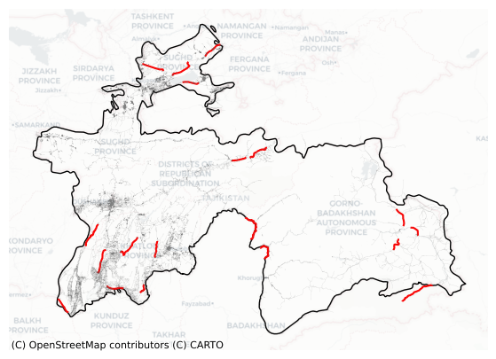
Find the locations of the twenty most damaged roads.
fig, ax = plt.subplots(1,1,figsize=(10, 5))

damage_results.to_crs(3857).sort_values('damage_corrected',ascending=False).head(20).plot(ax=ax,color='Red')
features.to_crs(3857).plot(ax=ax,facecolor="none",edgecolor='grey',alpha=0.5,zorder=2,lw=0.1)
world_plot.loc[world.SOV_A3 == country_iso3].plot(ax=ax,facecolor="none",edgecolor='black')
cx.add_basemap(ax, source=cx.providers.CartoDB.Positron,alpha=0.5)
ax.set_axis_off()
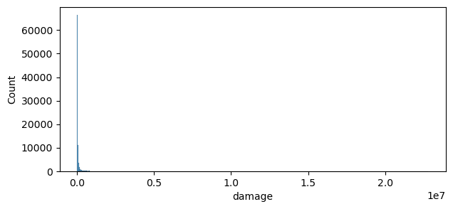
And create a distribution of the damages.
fig, ax = plt.subplots(1,1,figsize=(7, 3))

sns.histplot(data=damage_results,x='damage',ax=ax)
<Axes: xlabel='damage', ylabel='Count'>
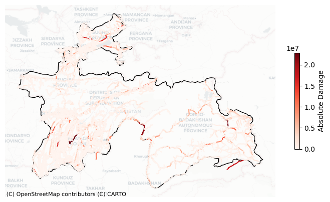
Plot all damages
fig, ax = plt.subplots(1,1,figsize=(10, 5))

damage_results.to_crs(3857).plot(ax=ax,column='damage_corrected',cmap='Reds',legend=True,
                   legend_kwds={'shrink': 0.5,'label':'Absolute Damage'},zorder=5)
features.to_crs(3857).plot(ax=ax,facecolor="none",edgecolor='grey',alpha=0.5,zorder=2,lw=0.1)
world_plot.loc[world.SOV_A3 == country_iso3].plot(ax=ax,facecolor="none",edgecolor='black')
cx.add_basemap(ax, source=cx.providers.CartoDB.Positron,alpha=0.5)
ax.set_axis_off()